Command Reference
Contents
1. File Formats
2. Command-line Programs
Data
Preparation:
Data
Analysis:
Building and Training HMMs:
Using
HMMs:
- parse [-p] <*.hmm>
<data.fastb>
- extract-motifs [options]
<trained.hmm> <num-motifs> <motif-length>
- motif-enrichment
<fastb-dir> <schema> <trackname>
<comma,separated,motif,list>
- get-likelihood [options]
<input.hmm> <training-dir>
- roc <in.gff> <out.roc>
<fastb-dir> <track-name> <min-signal>
<max-signal> <schema>
- roc-chain <*.hmm>
<fg-state> <bg-state> <site-size> <peak-size>
<fastb-dir> <track-name> <min-signal>
<max-signal> <jobID>
- sample [options] <in.hmm>
<out.fastb> <out.paths>
- scan-with-chains
<*.hmm> <fg-state> <bg-state> <threshold>
<window-size> <*.fastb>
- score-groups
<training-dir> <hmm> <fg-state> <bg-state>
<signal-track-name>
- summarize-paths.pl
<dir> <num-bins> <states>
Appendix A : HMM
File Format
File Formats
MUMMIE relies on several file formats; FASTB and schema files are
described in the section "Data Preparation Guidelines." Here we
describe several other formats used by MUMMIE.
1. TGF format
The TGF file simply specifies all possible dependencies between
continuous tracks. It's used to infer sparseness in the
covariance matrix of the multivariate Gaussian distributions that are
used to model the joint distribution of the continuous tracks.
The file begins with a numbered list of tracks, followed by a line
containing a "#", followed by a list of pairs of track numbers; these
pairs of track numbers specify which tracks have a nonzero
covariance. Every track must have a nonzero covariance with
itself.
Here's an example TGF file for a two-track data set:
1 PUM2-Signal
2 unpaired
#
1 1
1 2
2 1
2 2
In this case, a "complete graph" is assumed; i.e., all continuous
tracks covary. Discrete tracks are not included in the TGF file
(MUMMY assumes the discrete tracks are conditionally independent of all
other tracks, given the current state).
2. HMM format
The HMM file contains the complete specification of an HMM. You
don't want to edit HMM files directly, because they're
complicated. There are command-line programs (see below) that can
be used to manipulate parts of HMMs; you should use these programs
rather than trying to edit the HMM file directly.
3. HMMS format
The HMMS (HMM Structure) file specifies a metamodel, which is used to
merge multiple submodel HMMs together into one big HMM. This is
described below (see the program model-combiner).
4.
SUBMODELS format
The submodels.txt file specifies the HMMs to be merged together by the model-combiner program (see below
for a description of the file format).
Command-line Programs
• parse-ensembl.pl
> UTRs.txt
This program parses the file ensembl.txt in the current directory and
writes output to stdout. Don't run this program unless you know
what you're doing.
• par2fastb.pl
<outdir>
<lib1> <lib2> ...
This program parses the output of PARalyzer and generates the FASTB
files that MUMMIE uses as input. PARalyzer files must be
contained in the "raw" subdirectory of the current directory.
These include the normalization file (*.norm), the groups file
(*.groups), the distribution file (*.distribution), and the clusters
file (*.clusters), where all of these files have as their filestem the
library name.
• assemble-transcripts.pl
<indir> <outdir>
Whereas the par2fastb.pl
program generates FASTB files for individual exons, this program
assemblese those exons into transcripts, based on the transcript ID.
• get-folding-sequence.pl
<outdir>
This program extracts sequences having 200bp of
upstream context, to be used for folding of UTR sequences.
• kmeans
[options]
<training-dir>
<K>
options:
-n NUM = use at most NUM
training cases
-i NUM =
perform at most NUM iterations
-R epsilon
= stop when change in RSS<epsilon
-r NUM =
use NUM random restarts; keep best RSS solution
-s NUM =
use NUM iterations of random swapping upon convergence
-t =
tranpose the data matrix before clustering
-m = print
membership table
-c file =
write centroids into file
This program performs k-means clustering, which can be used
to try to identify the number of mixture components or number of states
to use in an HMM.
• random-HMM
[options] <num-states>
<connectivity[0-1]> <num-mixture-components>
<*.schema> <order> <outfile>
options:
-t *.hmm : use given
hmm as template for transition constraints
-s seed : use given
randomization seed
-c X : use canonical
topology of type X (I, II, III, IV, ...)
-u : use uniform
distribution for discrete chains
This program generates a random HMM with the specified number of states
and edge density (connectivity). The order parameter is for the
Markov chains used for discrete tracks (if any). The "canonical"
topologies are as shown in the following figure; they are useful as
starting points during exploration of new data:
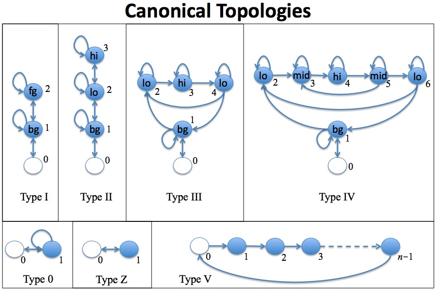
For example, you might start with a type 0 model and a type V model,
train these on background and binding-site sequences, respectively, and
then merge them into a composite model using the model-combiner program (see
below). Training is accomplished using the baum-welch program (see below),
though you can also edit individual parameters manually using the hmm-edit program.
• baum-welch
[options]
<initial.hmm> <dependency-graph.tgf> <training-dir>
<#iterations> <out.hmm>
options:
-B 0.3 = apply
"Bilmes sparsness", keep 30% of
entries
-c n = use n CPUs
-C file = center
& normalize data, save transforms to file
-d = use
diagonal covariance matrices
-g = use one
global cov matrix
-I = use
identity matrix and single coef for cov matrix
-l filename =
write log-likelihood curve to file
-L threshold =
stop when change in log-likelihood < threshold
-m file =
initialize means from cluster file
-M = do not
re-estimate means (requires -m)
-n V = add
gaussian noise with variance V
-N n = use at
most n training examples
-r = use one
global correlation matrix (re-estimate variances)
-R = do not
randomize initial HMM
-s seed = seed
randomizer with given seed value
-t file = tie
parameters according to profile in file
-u = update the
discrete emission chains during EM
This program trains an HMM using Expectation
Maxmization. A sample command line is:
MUMMIE/baum-welch assemble-model/combined.hmm nofold.tgf fastb 30
trained-combined.hmm -c 8 -l ll/combined.ll -n 0.0001 -R -t
combined-tie-profile.txt >> stdout/train-combined.stdout
• model-combiner
<meta-model.hmms> <submodels.txt> <outfile.hmm>
This program combines multiple HMMs into a single HMM. It does
this based on a "metamodel" topology, which is specified in the
"metamodel.hmms" file. The metamodel topology specifies the
transitions among the submodels, like this:
0 -> 1 : 1

1 -> 0 : 0.001

1 -> 1 : 0.9

1 -> 2 : 0.099

2 -> 2 : 0.9

2 -> 3 : 0.1

3 -> 3 : 0.9

3 -> 4 : 0.1

4 -> 4 : 0.9

  ...etc...
State 0 is the silent start/stop state; every other "state" in the
metamodel denotes a submodel. The mapping from metamodel "states"
to submodels is given by the submodels.txt file:
1 = bg-state.hmm

2 = low-state.hmm

3 = med-state.hmm

4 = hi-state.hmm

5 = trained-site-hi.hmm

6 = hi-state.hmm

7 = med-state.hmm

8 = trained-site-med.hmm
The program uses these files to merge the HMMs of the
submodels together into one big HMM. While all of the emission
distributions come from the submodels, the transition probabilities are
computed by compounding the between-submodel transitions (specified in
the metamodel file) with the appropriate transitions within the
submodels (i.e., transitions to or from the submodel's zero state), as
specified in section 6.6.2 of my book (Methods for Computational Gene
Prediction).
• hmm-edit
<in-out.hmm>
<operations>
This program allows you to change individual parameters of an
HMM. The program reads the specified HMM into memory, performs
the operations you've specified on the command line, and then writes
the modified HMM back into the same file. The operations are:
TRANS from to value : set transition
probability to
value
MIX state mixture_index value : set
mixture weight
to value
MEAN mixture_index track_index value :
set mean to
value
COV mixture_index track_A track_B value
: set
covariance to value
VAR mixture_index track_index value :
set variance
to value
TRK name :
add continuous track
COMP :
add another mixture component (applies to all states)
NMER state
track nmer prob : set P(last nmer base | prefix)
A state or index may be an individual value, comma-separated list (no
spaces), or the word ALL. You can specify multiple opererations
in a single command line, as in this example:
MUMMIE/hmm-edit bg-state.hmm TRANS 1 2 0.3 TRANS 1 4 0.7
• hmm-extract-state
<in.hmm>
<state#> <out.hmm>
This program extracts a single state from the given HMM and makes a new
HMM having only that state (plus the silent state 0). You can
specify "all" as the state# if you want to extract all states; each
state will then be extracted into a different file having the name
"filestem#.hmm" where # ranges from 1 to N and filestem is the third
argument to the program.
You can use this program to extract individual states from a trained
HMM and insert them into a new HMM with a more elaborate topology (for
example) using the model-combiner
program.
• install-chain
<*.chain>
<in.hmm> <out.hmm> <state>
This program installs a Markov chain into a particular state
in an HMM. You can also extract a chain from a state, using the
program extract-chain. This way, you can copy a chain from one
state to another, or from a state in one HMM to a state in another HMM.
• summarize-hmm
<in.hmm>
This program analyzes an HMM and prints out summary
information about it: the transition structure, the equilibrium state
distribution, the means of emission tracks, etc. It also attempts
to identify the "most foreground" state (the state having the hightest
mean for the first continuous track) and the "most background" state
(the state having the longest equilibrium duration).
•
motif-enrichment <fastb-dir> <schema> <trackname>
<comma,separated,motif,list>
options: -l = report logarithmic value
If I remember correctly, this program scans the FASTB files
in the specified directory for motif instances (exact matches).
You have to specify which track to scan.
• parse
[-p] <*.hmm>
<data.fastb>
options:
-p = use
posterior Viterbi
-g 2,3,4,5 =
emit gff, foreground is defined by state list
-P = just emit
posterior probabilities for all states
-d = second
parameter is a directory rather than a file
This program parses (or "segments") a FASTB file using an
HMM. With the -g option (recommended) it emits GFF elements
specifying where the foreground states are predicted to be
active. The -p option is also recommended; this causes MUMMIE to
use posterior probabilities during Viterbi decoding, which in many
cases can give more accurate predictions.
• extract-motifs
[options]
<trained.hmm> <num-motifs> <motif-length>
options:
-s X = state X
only
-L B = use state
B as a background, compute LL ratios
-a = auto-detect
foreground state, use LL ratio
-i = increment
state number along length of motif
-l F = score
strings from list file F
This program enumerates the highest-scoring nmers under a
given state's Markov chain. This is useful if you've just run
baum-welch (EM) and are hoping that one of the states will have
captured sequence biases of particular regions in the input
files. Use -s to specify the state; you should also use -L to
specify a background state (ranking is then by likelihood ratio).
• fastb-stats
[options]
<*.fastb>
<*.schema>
options: -d = filename is actually a directory
This program gives some statistics about FASTB files.
• extract-chain
<*.hmm>
<state>
This program extracts the Markov chain from a given state;
the first discrete track is assumed to be the chain of interest.
•
fastb-length [options] <*.fastb> <*.schema>
options: -d = filename is actually a directory
This program checks that all tracks in a FASTB file have the
same length (which they should), and reports that length.
•
fastb-add-folding-noave.pl <indir-fastb> <indir-fold>
<outdir>
This script adds folding probabilities (probability of being
unpaired) from RNAplfold into FASTB files as an additional track.
•
fastb-extract-tracks.pl <in.fastb> <out.fastb>
<track1> <track2> ...
This script extracts the specified tracks from a FASTB file.
•
fastb-to-fasta.pl <in.fastb> <out.fasta>
This program converts a FASTB file to FASTA by keeping only
the discrete tracks.
•
cat file | fastb-to-xgraph.pl
This script graphs the continuous tracks of a FASTB file,
using the program xgraph.
•
get-likelihood [options] <input.hmm> <training-dir>
where: -p "0 1 3 2 5 6 4" = apply specified state mapping
This program computes data likelihood for a given HMM.
•
get-schema.pl <fastb-dir>
This program infers a schema from a directory of FASTB files.
•
roc <in.gff> <out.roc> <fastb-dir> <track-name>
<min-signal> <max-signal> <schema>
This program computes the area under an ROC curve, so that
the predictions in a GFF file can be evaluated. It does this by
looking at the specified track-name in the FASTB files and slicing them
at many different thresholds. Each slicing threshold effectively
segments that track into contiguous intervals, which are compared to
the predicted intervals in the GFF file, to compute sensitivity and
false positive rate. Each slicing threshold thus gives rise to
one point in an ROC curve.
•
roc-chain <*.hmm> <fg-state> <bg-state>
<site-size> <peak-size> <fastb-dir>
<track-name> <min-signal> <max-signal> <jobID>
options:
-w
file = also construct roc curve for
PWM in file
-b
file = use background chain in file for PWM
-r
file = write curve into file
-p =
evaluate via peaks rather than uniform slices
This program is similar to the "roc" program, but it uses a
Markov chain to perform prediction (ignoring all continuous tracks).
•
sample [options] <in.hmm> <out.fastb> <out.paths>
options:
-m <min-length>
-M <max-length>
-r <randomization-seed>
-S X = stay in state X
-D = discrete tracks only
-R N = repeat sampling N times
This program samples FASTB sequences from an HMM; this is
useful for simulations.
•
scale-data [options] <input-dir> <transforms.out>
<schema.txt>
option: -n V = add gaussian noise (after scaling) with
variance V
This OBSOLETE program scales the continuous tracks in a set
of FASTB files. It is no longer needed, because par2fastb.pl now
scales the data so that the maximium value is 1 and the minimum is 0.
•
scan-with-chains <*.hmm> <fg-state> <bg-state>
<threshold> <window-size> <*.fastb>
This program scans FASTB files with a pair of Markov chains
and emits intervals with a sufficiently high likelihood ratio.
•
score-groups <training-dir> <hmm> <fg-state>
<bg-state> <signal-track-name>
This program scores PARalyzer groups.
•
smooth-fastb [ops] <in.fastb> <window-size>
<#iterations> <out.fastb>
where: -t abc,xyz,... = smooth only the listed tracks
This program smooths FASTB files. It is OBSOLETE.
•
smooth-all.pl <in-dir> <out-dir> <window-size>
<#iterations> [tracks]
This program smooths FASTB files. It is OBSOLETE.
•
split-train-test.pl <indir> <num-partitions>
<dir-stem>
This program can be used to split a directory into separate
training and test sets.
•
subset-fastb <in.fastb> <track,track,...> <out.fastb>
This program extracts the specified tracks from a FASTB file.
•
summarize-paths.pl <dir> <num-bins> <states>
I don't remember what this program does.
•
discretize <in.schema> <input-dir> <num-bins>
<boundaries.out> <out.schema>
This program discretizes the continuous tracks in FASTB
files.
•
threshold <in.schema> <input-dir> <threshold>
This program applies a threshold to FASTB files.
• extract-gff-intervals
<in.gff> <fastb-dir> <schema> <out-dir>
This program reads the intervals given in the GFF file and then
extracts the sequences for those intervals from the corresponding FASTB
files. The "substrate" field of the GFF lines specifies the
filestem of the FASTB file that contains the interval.
•
train-state-labels [options] <input.hmm> <training-dir>
<output.hmm>
where: -p "0 1 3 2 5 6 4" = apply specified state mapping
This program is OBSOLETE.
• motif-scan.pl <motifs.fasta>
<fastb-dir> <ignore-margin>
This program searches the fastb files in the <fastb-dir> for
motif occurrences, where the motifs are specified in
motifs.fasta. The <ignore-margin> parameter specifies a
margin at the beginning and end of each sequence to ignore.
• fastb-extract-tracks-dir.pl
<indir> <outdir> <track1> <track2> ...
This program processes all of the FASTB files in the directory
<indir>. For each file, it makes a new version of the file
in <outdir> that contains only the tracks listed on the command
line.
• fasta-to-fastb.pl <in.fasta>
<in.schema> <out-dir>
• change-track-name.pl
<old-track-name> <new-track-name> <fastb-dir>
•
•
This program performs a numerical subtraction between a track in one
set of files and another track in another set of files. After the
subtraction, the specified threshold is applied to the resulting track;
any value below the threshold is set to zero.
• longest-utr-per-gene.pl
<in-dir> <out-dir>
This program assumes each file in the directory <in-dir> has a
name of the format GENE_ISO.FASTB, where GENE is the gene ID and ISO is
an isoform number. The longest isoform for each gene is copied to
the directory <out-dir>
• make-tgf.pl
<schema.txt> <full|diag> <outfile.tgf>
This program makes a TGF file based on the given schema. Specify
full for a full covariance matrix, or diag for a diagonal covariance
matrix.
• parse-clusters.pl <clusters.csv>
This program parses a PARalyzer clusters file to produce a GFF file
giving the locations of "clusters" (also called "interaction sites").
• fastb-to-gff.pl <in.fastb>
<out.gff> <trackname> <threshold>
This program applies the given threshold to a FASTB file, identifies
the intervals scoring over the threshold, and writes those intervals
into the output file.
• get-groups.pl <main-track>
<fastb-dir> <extra-margin>
This program finds the "groups" (continuously nonzero intervals) in a
set of FASTB files, adds the specified margin to the beginning and end
of each interval, and writes the interval coordinates to stdout in GFF
format.
• positions-relative-to-peak.pl
<peaks.gff> <sites.gff>
• find-peaks
[options] <*.fastb> <*.schema> <track-name>
where: -d = filename is actually a directory
-t T = apply
threshold T (default=0.1)
-g W = emit
histograms around peak (+/- width W)
This program finds the peaks in a given track for a single FASTB file
or a directory of FASTB files and writes the output in GFF format to
stdout.
• get-extrema <fastb-dir>
<schema.txt> <track-name>
This program reports extrema for a given track
in a set of FASTB files.
Appendix A : HMM File Format
The file begins with a header section that gives the number of states
and specifies the data types for the emissions:
47 states
schema:
1 1
DNA
ACGT
AGO-Signal |
The first line gives the number of states. The second line
contains the word "schema" followed by a colon. The third line
contains two numbers: the number of discrete data tracks, and the
number of continuous data tracks. This is followed by a list of
discrete data tracks. For each discrete data track, give the name
and the alphabet, on separate lines. In the example above, DNA is
the name of the discrete data track and ACGT is the alphabet for that
track. After all of the discrete tracks, list the continuous
tracks, one per line.
The next section gives the transition matrix:
transitions:
8 8
0
0
0
0
0
0
0 1
1
0
0
0
0
0
0 0
0
1
0
0
0
0
0 0
0
0
1
0
0
0
0 0
0
0
0
1
0
0
0 0
0
0
0
0
1
0
0 0
0
0
0
0
0
1
0 0
0
0
0
0
0
0
1
0
|
The first line of this section gives the transitions keyword and a
colon. The next line gives the dimensions of the matrix; the
matrix must be square and the dimension should be the number of
states. In this example above we're dealing with an 8-state
HMM. The matrix follows, with each row giving the transition
probabilities into each state. That is, row N of the matrix gives
the transition probabilities into state N. For the example above,
the only state that can transition into state 0 is state 7, the only
state that can transition into state 1 is state 0, etc. Don't
forget that rows give transitions into each state, not transitions out
of that state!
The remaining sections specify the emission probabilities for each
state, in order, starting with state 1 (since state 0 is silent and
therefore has no emissions). Here's an example:
state 1 emissions:
2
0.2 0.8
1 1e-07
1 1
0.01
1 0.5
1 1
0.01
1 order
alphabet:
ACGT
A -2.15176
C -1.3633
G -1.27629
T -1.05315
AA -2.48491
AC -1.38629
AG -1.38629
AT -0.875469
CA -0.980829
CC -2.07944
CG -2.07944
CT -0.980829
GA -inf
GC -1.0116
GG -1.29928
GT -1.0116
TA -2.48491
TC -1.38629
TG -0.875469
TT -1.38629
|
After the header line ("state 1 emissions:") is a section that
gives the multivariate gaussian distribution for the continuous
emission tracks. The line after the header staes the number of
mixture components (2 in this example). The next line gives the
mixture weights for this state (0.2 and 0.8 here). Next comes the
parameters for the first mixture component. The first line ("1
1e-07") gives the vector of means for the multivariate distribution;
the first number on the line says how many elements are in the vector,
and the remaining numbers on the line give the vector elements (the
means for the continuous tracks, in the same order that those tracks
are listed in the schema section at the top of the file). After
this is a line with two numbers ("1 1") in this example; these
give the dimensions of the covariance matrix, which is always a square
matrix (so the two numbers will always be equal). In this case
the covariance matrix is 1x1 because there is only one continuous track
in this example. The lines that follow give the rows of the
covariance matrix. In this case there's only one line (because
the Cov matrix is 1x1) and that line gives the variance of the single
continuous track. After this we just have another mixture
component specification; in this example, that second mixture component
has a mean of 0.5 and a variance of 0.01.
Finally, each state's discrete emission distribution is given, as a
Markov chain. First we give the order of the chain ("1 order" in
this case), followed on the next line by the keyword "alphabet:" and
then the actual alphabet letters on the next line after that ("ACGT" in
this example). After this we have the list of N-mers and their
emission probabilities in log space. For N-mers longer than 1
symbol, the log value is a conditional probability: the probability of
the last base of the N-mer conditional on the preceding
(N-1)-mer. For example, the line "CCTG -1.23"
would mean that P(G|CCT)=0.2923.