Intro to Multivariate Markov Modeling

Multivariate Markov modeling is potentially useful any time you have a multivariate sequence—i.e., an ordered sequence of observations, with each observation consisting of measurements from some fixed set of variates (each of which may be numeric or categorical).  A prime example is a genomic sequence for which we have several covariates sampled at each nucleotide in the sequence—e.g., the methylation status of that nucleotide, the number of sequencing reads aligned to that position from a sequencing assay, some measure of evolutionary conservation of that residue across a particular phylogeny, etc.  The figure below shows a hypothetical example including one discrete variate (DNA sequence) and four continuous variates: 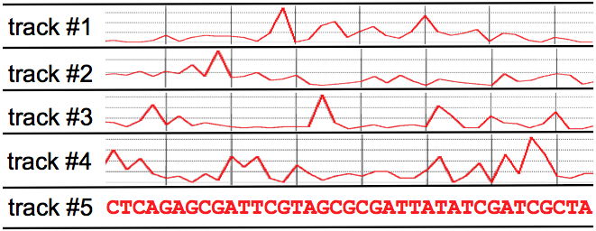We can thus think of a multivariate sequence as being represented by a matrix, with the rows corresponding to tracks (variates) and the columns corresponding to observations (sequence indices).  Further, we can imagine the matrix being generated one column at a time, via a temporal process.  Thus, the first sequence position (matrix column) would be generated at time 0, the second position at time 1, and so on.  In this way, the sequence comprises an ordered set of multivariate observations (matrix columns), with successive observations in the sequence coming into existence at successive points in time.  That is, we can pretend that the sequence represents a multivariate time series (even if the data wasn't actually generated by a temporal process). 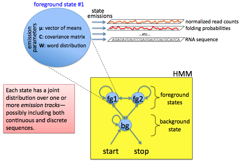We thus posit an abstract machine, called a multivariate Markov model (MMM), which we presume to have emitted the sequence(s) of interest, from left to right, during the time evolution of the machine.  At any given time the machine is in some state, which is chosen from a finite set of discrete states, Q = {q0, q1, ..., qm}. The machine starts in state q0 and stochastically transitions from state to state.  At each time unit the machine emits a multivariate observation and then transitions to another (possibly the same) state.  When the machine eventually transitions back into state q0, that run of the machine is over, and we have a complete observation sequence.  We can of course start up the machine again, in which case it will again begin in state q0, follow some random trajectory of states over time, producing another multivariate observation sequence, and and then terminate when again it randomly enters state q0.  Successive state paths and the multivariate emission sequences produced by different runs of the machine will generally be different, since the operation of the machine is stochastic. The stochastic nature of the machine is characterized by a set of probability distributions that bias the machine's behavior.  These include emission distributions and transition distributions.  The transition distributions govern how the machine transitions from state to state: given that the machine is currently in state qi, the next state, qj, is chosen according to qj ~ P(q|qi).  Similarly, given that the machine is in state qi at time k, the multivariate observation yk emitted during this time unit will be chosen according to yk ~ P(y|qi), where yk is an n-dimensional vector.  Note that state 0 is a special silent state (it has no emissions); every run of the machine begins and ends in this state, so that every state path executed by the state begins and ends with state 0, and state 0 can only occur at the beginning and ending of valid state paths. Now suppose that the machine has just completed a run, emitting a series of multivariate observations S = y0y1...yL-1 of length L.  In producing this sequence S of observables, the machine must have visited a series of states φ = q0x0x1...xL-1q0 of length L+2 (since the q0 at the beginning and end of the path emit nothing).  This state path φ is unobservable.  This is unfortunate, because knowing the path used by the model to generate the observation sequence would allow us to parse the sequence into meaningful segments.  Consider an example HMM with four states colored blue, orange, red, and green.  The following figure shows a hypothetical nine-dimensional observation sequence emitted by this HMM: 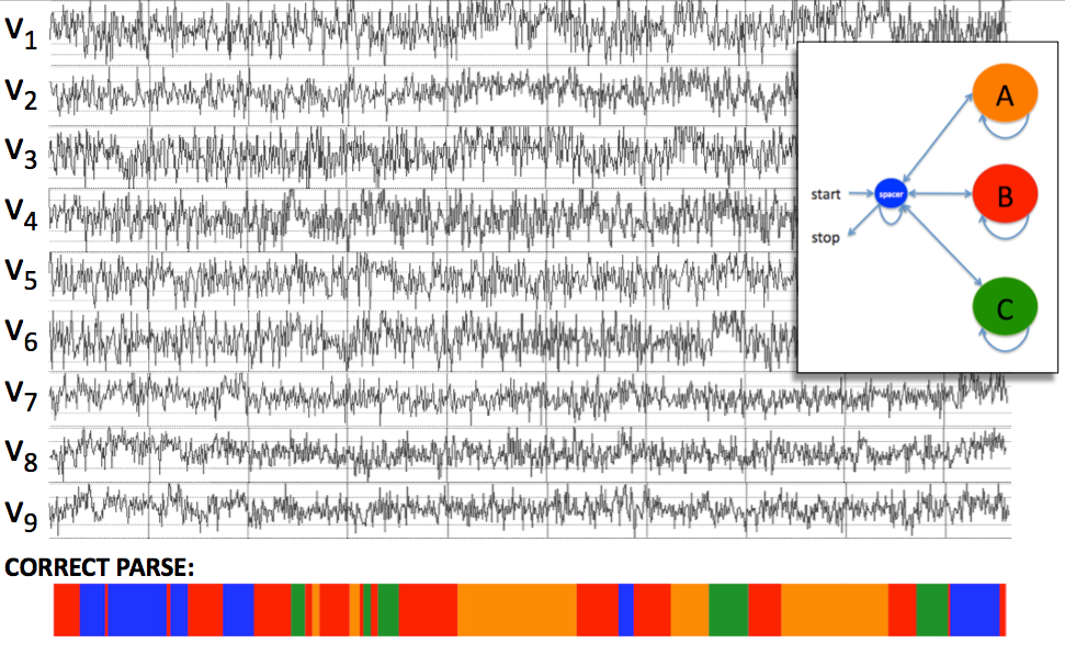The bottom row of colored stripes shows the actual path followed by the HMM when it generated the observation sequence--i.e., orange segments indicate when the machine was in the orange state, red segments denote when the machine was in the red state, etc.  Since we don't know the actual state path followed by the machine when it generated this sequence, the best we can do is to make inferences about probable paths that would generate this sequence.  If we knew the parameters of the model (the emission and transition probability distributions) we could make such inferences. Now suppose that we have a multivariate sequence produced not by an MMM but by some biological experiments.  Even though the sequence was not emitted by an MMM, we might pretend that it was emitted by some MMM.  If we can find an MMM with an appropriate state space and appropriate parameters (emission and transition distributions), then making inferences about probable paths for that MMM to emit this sequence could be useful, in that it gives us a way to parse the sequence into segments corresponding to different states of the MMM.  If our model does in fact accurately capture the statistical structure of the class of biological sequences we're modeling, then the parses that we infer for those sequences using this model may be useful.  This is the same modeling paradigm that has been successfully applied for finding genes and other functional elements in genomic DNA using hidden Markov models (HMMs); the only difference is that MMMs emit multivariate sequences instead of just a univariate DNA sequence. Thus, the goal in multivariate Markov modeling is to find a suitable model (an MMM) that captures the statistical characteristics of the multivariate sequences for which we'd like to make inferences.  This involves choosing a state space (a set of labels that we'd like to apply to individual sequence positions), a state topology (a set of rules dictating which states may immediately follow which other states in a valid state path), and a set of parameters specifying the emission and transition distributions for the model.  Note that the state topology and the transition distributions impose a grammar on the sequences: they specify the ways in which functional elements (invervals of sequence emitted by a single state) can occur in a sequence, in terms of their ordering, their spacing, and their lengths.  Thus the first step in multivariate Markov modeling is to choose a set of labels and to inventory everything you know about how functional elements in your sequences relate to each other.  For example, in a gene-finding model the labels could be {exon, intron, intergenic} and the grammar rules would be: intergenic → intergenic intergenic → exon exon → exon exon → intron inron → intron intron → exon exon → intergenic Note that there is no rule inron → intergenic, because an intronic nucleotide is never followed by an intergenic nucleotide in a genomic annotation.  Now you can assign your labels to individual states, and for each rule A → B you can create a transition from state A to state B.  You now have a model structure, but it needs to be trained, meaning that you need to learn parameters for the emission and transition distributions.  Methods for doing this are detailed in the Modeling Guidelines page. Once your model is trained you can then apply it to sequences in various ways.  You can parse the sequence as done in the examples above to obtain a most probable parse (using Viterbi decoding).  Alternatively, you can compute posterior probabilities for the existence of a functional element of a given type spanning a given interval of sequence (methods for doing this are detailed on the Commands Reference page).  You can also train multiple models--one for each of several classes of sequence--and then classify novel sequences by computing the likelihood of each sequence under each model and assigning the sequence to the model for which it has the highest likelihood (or the highest posterior probability if you can assign reasonable class priors).  There are still other possibilities, including motif finding, clustering, and analyses of element co-occurrence or positional preferences; methods for performing these and other types of analyses will be detailed here in the near future.

contact